At the same time LLMs are changing the world, we have witnessed fast progress in AI image and video generation. AI models are now able to synthesis high quality, high fidelity and high resolution images via text prompting. Mainstream generative model architectures have shifted from VAEs, flows and GANs to diffusions and transformers. In this post I take notes of several vision models. It may be regularly updated to reflect latest research development.
Vision Understanding
ViT
Vision Transformer (ViT) ( Citation: Dosovitskiy, Beyer & al., 2020 Dosovitskiy, A., Beyer, L., Kolesnikov, A., Weissenborn, D., Zhai, X., Unterthiner, T., Dehghani, M., Minderer, M., Heigold, G., Gelly, S. & (2020). An image is worth 16x16 words: Transformers for image recognition at scale. arXiv preprint arXiv:2010.11929. ) applies the transformer architecture to vision inputs. Images are segmented to patches, and the patches are embedded as sequence of vectors, with patch ordering as position embedding. The figure below illustrates the architecture. The model achieves superior performance than convolutional neural networks (CNNs) in many tasks, and has become a basic component in other subsequent vision models. Refer to @lucidrains/vit-pytorch for a simple implementation of ViT.
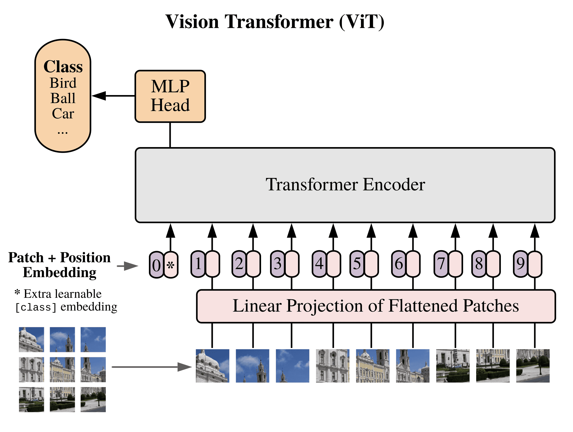
ViT architecture. Source: Machine Learning Mastery
CLIP
CLIP ( Citation: Radford, Kim & al., 2021 Radford, A., Kim, J., Hallacy, C., Ramesh, A., Goh, G., Agarwal, S., Sastry, G., Askell, A., Mishkin, P., Clark, J. & (2021). Learning transferable visual models from natural language supervision. PMLR. ) is a foundational model developed by OpenAI that set the stage for multi-modality modeling. Traditionally, image classification models were trained to map input to a fixed set of classes, which is inflexible. By jointly training text and image embeddings on massive natural text and image pairs, CLIP models learn associations of images with texts, which allows it to perform open-set classification.
Architecture
The CLIP model consists of a text encoder and an image encoder, trained on large collection of (text, image) pairs. For image encoder, two architectures are experimented, ResNet and ViT, and ViT was found to perform better than ResNet. The text encoder is a Transformer, the base one has 12 layers and 512 embedding dimensions, for a total of 63M parameters, with a vocab size 49152, and sequence length capped at 76.
Dot product between text embedding and image embedding of a pair $(T_i, I_i)$ is maximized, and dot product for pairs $$ \{(T_i, I_j)\}_{j\neq i} $$ and $$ \{(T_j, I_i)\}_{j\neq i} $$ are minimized, where $I_j$ and $T_j$ are other texts and images in the same batch. A large batch size of 32768 is used in the paper. In the figure below, this means maximizing cross entropy of the first row ➕ cross entropy of the first column, cross entropy of the second row ➕ cross entropy of the second column, and so on.
[Further Detail] The text sequence is bracketed with
[SOS]and[EOS]tokens and the activations of the highest layer of the transformer at the[EOS]token are treated as the feature representation of the text which is layer normalized and then linearly projected into the multi-modal embedding space.
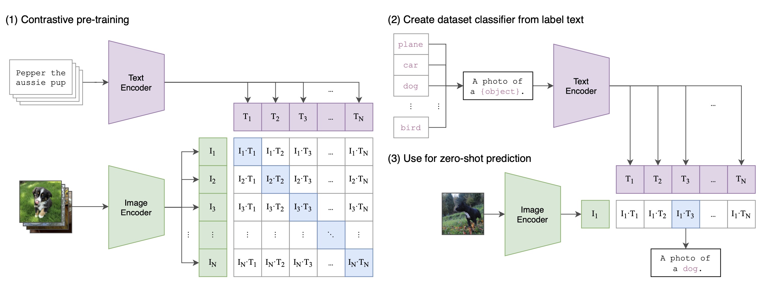
CLIP model architecture. Source: paper
Training
- Dataset. 400 million non-open (text, image) pairs.
- Loss. The loss is cross entropy loss that maximizes probability for (text, image) pairs in the training data and minimizes probability for not-paired texts and images in training batches. The paper provided the following pseudocode:
| |
- Code. huggingface - CLIP
Note that CLIP is a discriminative model. It can be used for image search and zero-shot image classification, but it is not a generative model, and it cannot be directly used to generate images. It is often served as a text encoder component in many image generation models.
MAE
Masked Autoencoder (MAE) ( Citation: He, Chen & al., 2022 He, K., Chen, X., Xie, S., Li, Y., Dollár, P. & Girshick, R. (2022). Masked autoencoders are scalable vision learners. ) is a ViT-based denoising autoencoder that learns image representations. 75% patches of training images are masked and the objective is to reconstruct the masked pixel values, with MSE between predicted vector of pixels and original pixel values as loss. The encoder is a ViT model that is only applied to unmasked patches. The decoder is a smaller ViT model that is only used for reconstruction during training, but is discarded afterwards since only encoder outputs are used in downstream tasks.
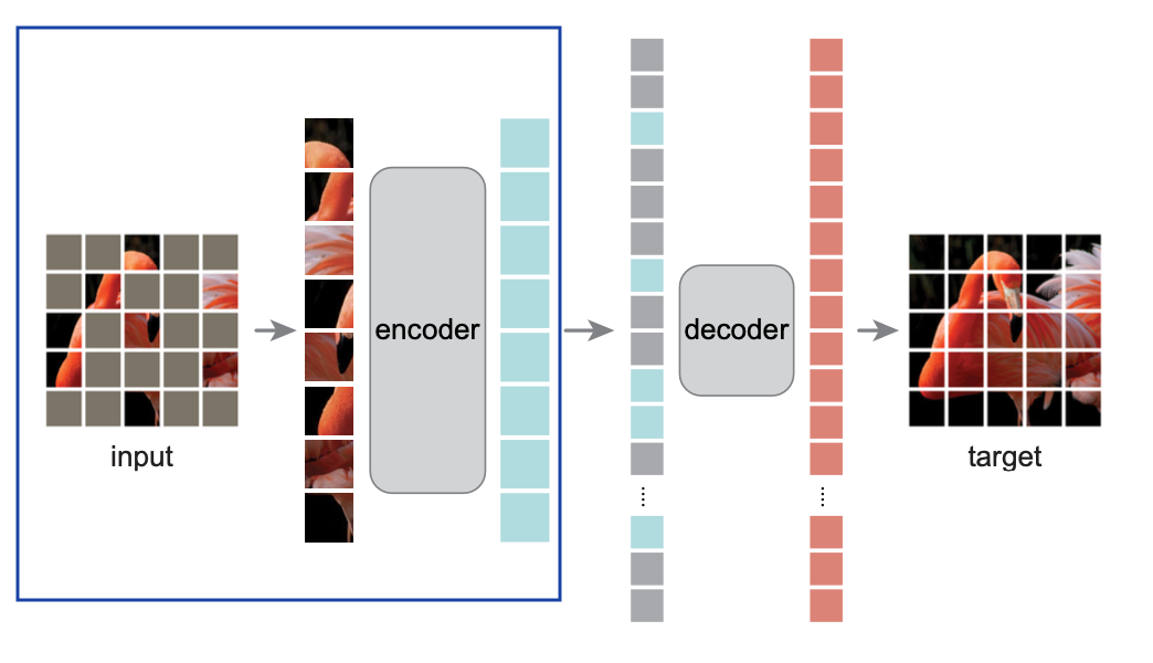
MAE model architecture. Source: paper
SAM
Segment Anything (SAM) is an interactive image segmentation model released by Meta AI. The model can be used for image and video editing, and can also be integrated into AR/VR headset to select objects.
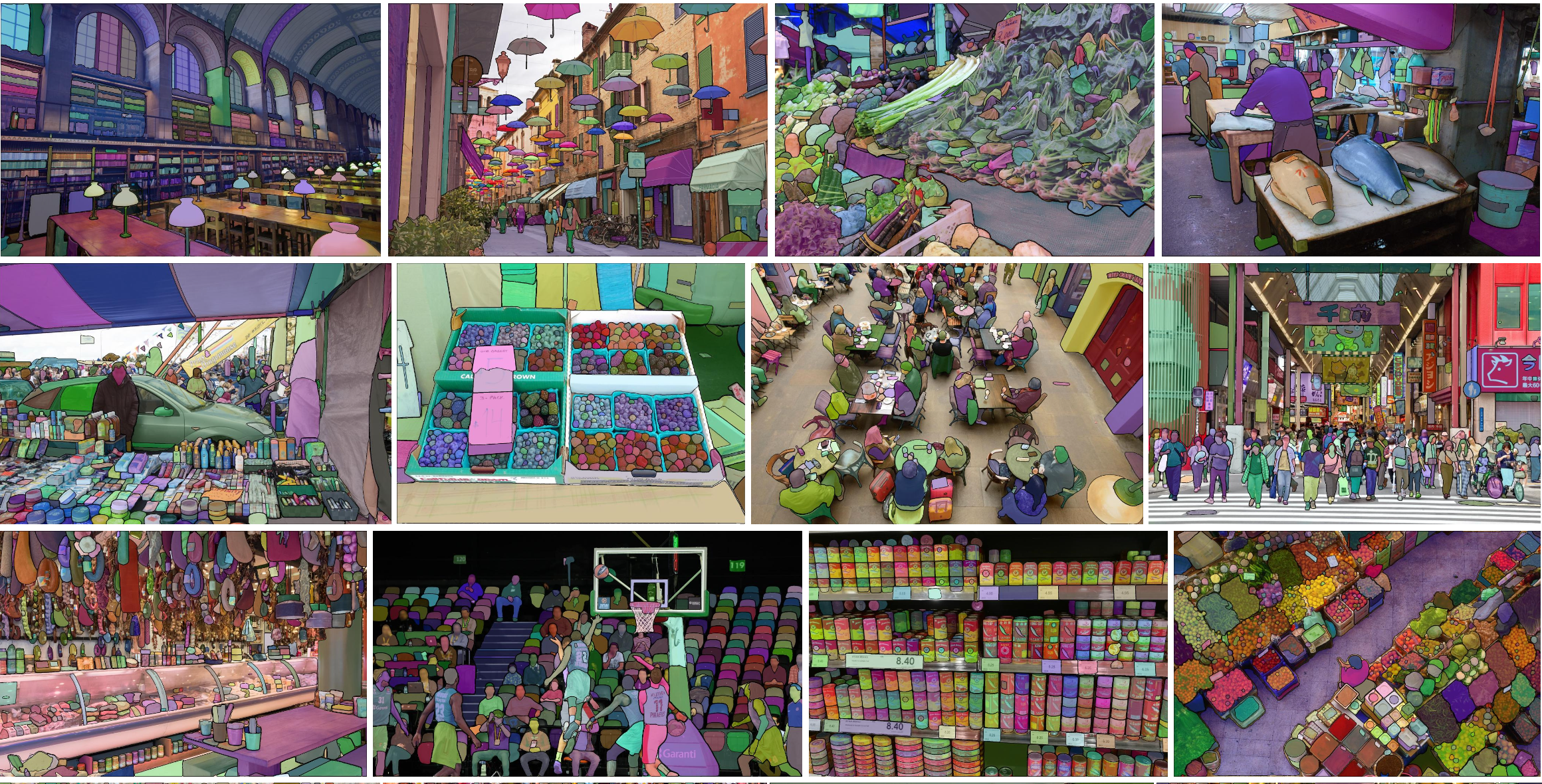
Source: paper
Architecture
SAM consists of a one-time image encoder, a prompt encoder and a lightweight mask decoder. The image encoder is a ViT model that produces embedding for an input image. It has 632M parameters, which takes ~0.15 seconds to run on an NVIDIA A100 GPU. The prompt encoder maps points, boxes and texts via CLIP and CNNs. The decoder is a transformer that predicts object masks from image embeddings and prompt embeddings. The prompt encoder and mask decoder have 4M parameters, and take ~50ms on CPU in the browser.
Note that the model only predicts binary masks, but not labels (chairs, cars, etc.). SAM model architecture. Image embedding can be computed once per image in the backend on GPUs. After the embedding is obtained, masking prediction can run very fast in the browser, which enables real-time interactive prompting. Source: https://segment-anything.com
Training
- Dataset. The model is trained on 11M images with 1B+ masks. The dataset called SA-1B is released here along with the model.
- Loss. Mask prediction is supervised with linear combination of focal loss ( Citation: Lin, Goyal & al., 2017 Lin, T., Goyal, P., Girshick, R., He, K. & Dollár, P. (2017). Focal loss for dense object detection. ) and dice loss ( Citation: Milletari, Navab & al., 2016 Milletari, F., Navab, N. & Ahmadi, S. (2016). V-net: Fully convolutional neural networks for volumetric medical image segmentation. Ieee. ) . The focal loss is a modulated cross entropy loss: $$ \mathrm{FL}(p) = -\alpha(1-p)^\gamma\log(p). $$ The dice loss measures overlap between predicted and ground-truth labels. Let $y_i$ denote label, the formula is $$ \mathrm{Dice}(p) = 1 - \frac{2\sum y_i\cdot p_i}{y_i^2 + p_i^2+1} $$
- Hardware. The model was trained for 3~5 days on 256 A100 GPUs.
More details can be found at https://segment-anything.com/.
Image Generation via Discrete Tokenization
VQ-VAE
VQ-VAE ( Citation: Van Den Oord, Vinyals & al., 2017 Van Den Oord, A., Vinyals, O. & (2017). Neural discrete representation learning. Advances in neural information processing systems, 30. ) is a seminal paper published by Google DeepMind researchers in 2017. VQ-VAE is a way to regularize the latents, by forcing the decoder to only allocate probability mass to a finite set of learned vectors. The model was proposed to address the “posterior collapse” issue in VAEs, which is the phenomenon that the decoder often ignores the latents, producing blurry and monotonous images.
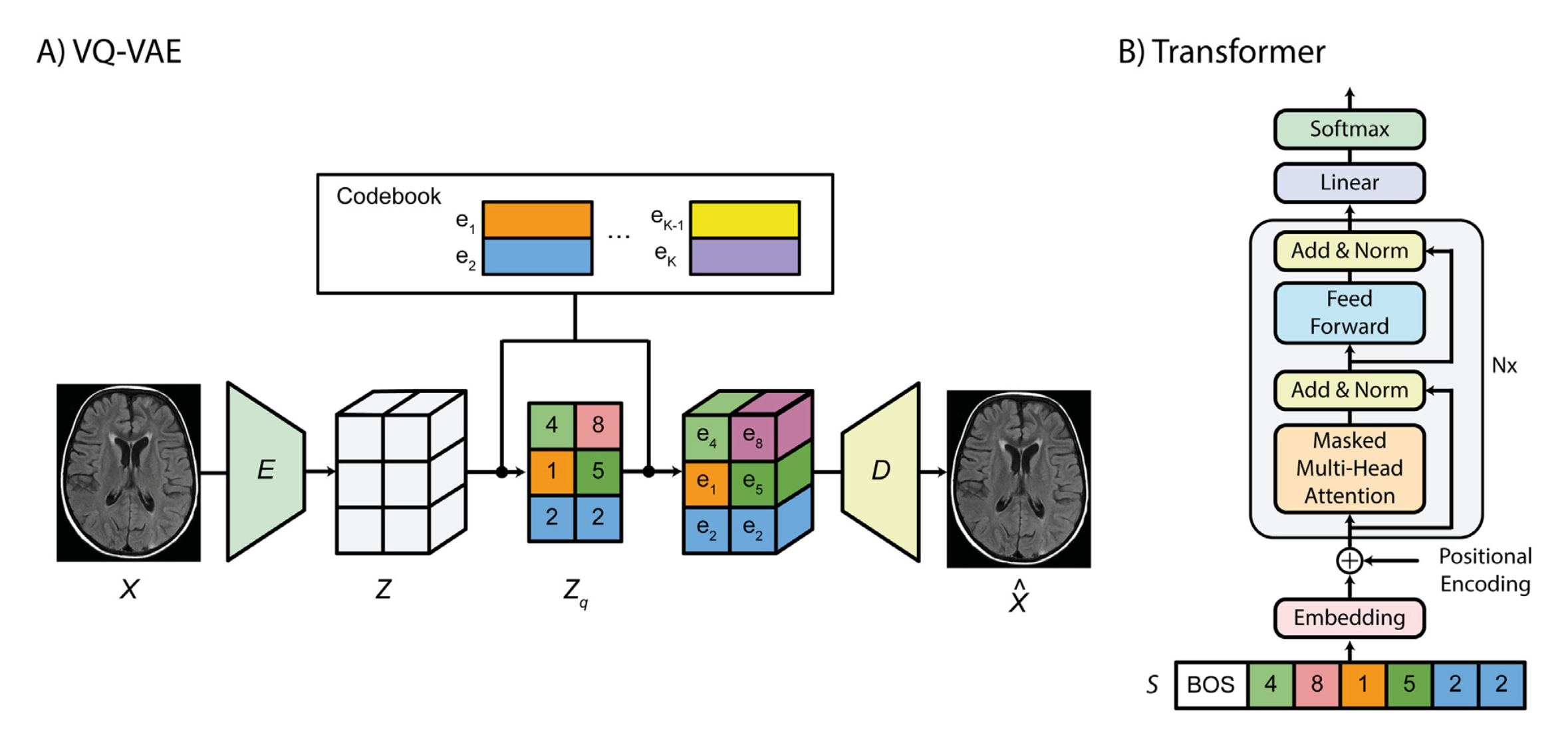
VQ-VAE Architecture. Source: ResearchGate
VQ-VAE consists of two parts: an autoencoder that learns discrete representation of images, and an autoregressive model that learns to generate latents. The encoder maps input images of shape $H\times W\times C$ to tensor $z$ of shape $h\times w\times c$. The downsampling factor $f=H/h=W/w$ is often set to $8$ or $16$. The latent codes in codebook, which serve as input to the decoder, are also designed to have the same channel dimension $c$. As clearly illustrated in the figure above, in forward pass, each spatial element in $z$ is mapped to its closest latent $e_i$ from the codebook $\{e_1,\ldots,e_K\}$ by computing Euclidean distances. However, in backward pass, we need to consider how to back-propagate gradients through this discrete operation. The proposal is simple: just copy the gradient of $e_i$ from the right side to the left side. Since we want the encoder outputs to be close to their learned embeddings, this strategy should be a useful way to adjust the the encoder outputs.
The loss function for training the autoencoder is
$$ \ell = \log p(x\mid z_q(x)) + \|sg[z_e(x)] - e\|^2 + \beta\cdot\|z_e(x) - sg[e]\|^2, $$
where sg stands for “stop gradient” and it is the .detach() operation in PyTorch. This means, for the second term, we only update the embedding vector $e$, treating $z_e(x)$ as a constant; for the third term, we only update $z_e(x)$, treating $e$ as a constant.
Here is a breakdown of the three terms:
- The decoder optimizes $\log p(x\mid z_q(x))$ only.
- To make sure the encoder commits to an embedding and its output does not grow, a commitment loss is added as the third term. The encoder optimizes $$ \log p(x\mid z_q(x)) + \beta\cdot\|z_e(x) - sg[e]\|^2. $$
- The embeddings are optimized by the middle term $\|sg[z_e(x)] - e\|^2$.
Note that under the assumption that the decoder output is Gaussian: $$ p(x\mid z_q(x)) \sim e^{-\|x-\mu\|^2}, $$ the first loss term reduces to mean squared error (MSE) loss. So when it comes down to implementation, the loss is directly implemented as $$ \ell_{\mathrm{VQ-VAE}} = \ell_{recon} + \ell_{codebook} + \beta\cdot\ell_{commit} $$ with $$ \ell_{recon} = \|x-\hat{x}\|^2,\quad \ell_{codebook} = \|sg[z_e(x)] - e\|^2,\quad \ell_{commit} = \|z_e(x) - sg[e]\|^2. $$
The encoder and decoder used in the original VQ-VAE paper are CNNs, and after the autoencoder is trained, an autoregressive model (PixelCNN) is learned to autoregressively generate tokens in the latent space. Nowadays, the PixelCNN model has been substituted with transformers. In the original experiment, x = 128 x 128 x 3 images are mapped to z = 32 × 32 × 1 tensors, and the codebook consists of K=512 vectors each of dimension 1. This means that each each of the 32 x 32 = 1024 latent value comes from one of 512 values.
Below are two open-source PyTorch implementations of VQ-VAE:
VQ-VAE can be used to generate images: first generate tokens in latent space by the trained generative model, then use the decoder to map generated latents to pixel space. An important architectural improvement, the VQ-GAN model, successfully substituted PixelCNN with transformers, and helped further popularize the approach.
VQ-GAN
VQ-GAN ( Citation: Esser, Rombach & al., 2021 Esser, P., Rombach, R. & Ommer, B. (2021). Taming transformers for high-resolution image synthesis. ) is an improvement over the VQ-VAE model, at a time when the Transformer architecture became popular. Here are the differences:
- The PixelCNN model used in the VQ-VAE paper to generate tokens in latent space is replaced by a Transformer, though the training objective is still autoregressive, i.e. the latent tensor is flattened to a 1D vector and the model is trained to predict the next token given all previous tokens. The encoder and the decoder are still CNNs.
- The MSE loss $\|x-\hat{x}\|^2$ used in VQ-VAE is replaced with a “perceptual loss”, meaning that MSE is calculated between feature maps $\|f(x)-f(\hat{x})\|^2$ for some CNN model $f$, instead of between original images in pixel space. Further, a GAN objective is added to the original VQ-VAE objective: $$ \ell_{GAN} = \log D(x) + \log(1 - D(\hat{x})) $$ where $D$ is a patch-based discriminator. The complete objective is $$ \ell = \ell_{\mathrm{VQ-VAE}} + \lambda\cdot\ell_{GAN} $$ where $\lambda$ is a dynamically-adjusted weight (refer to paper for detail).
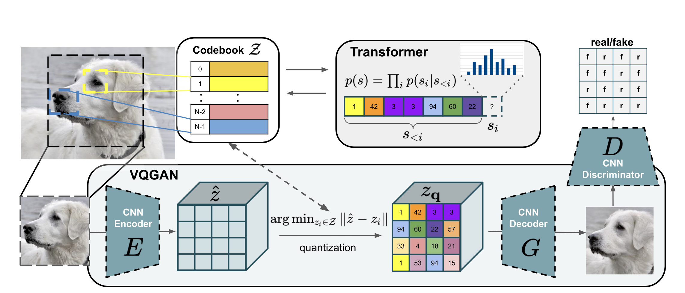
VQ-GAN Architecture. Source: paper
Recently, Google’s series of work that are built upon the VQ-GAN model demonstrated the potential of masked token modeling approach to visual content generation. The approach is to learn an autoencoder tokenizer to map images or videos to discrete tokens, then train a transformer model for masked token prediction. Here we briefly mention some of them.
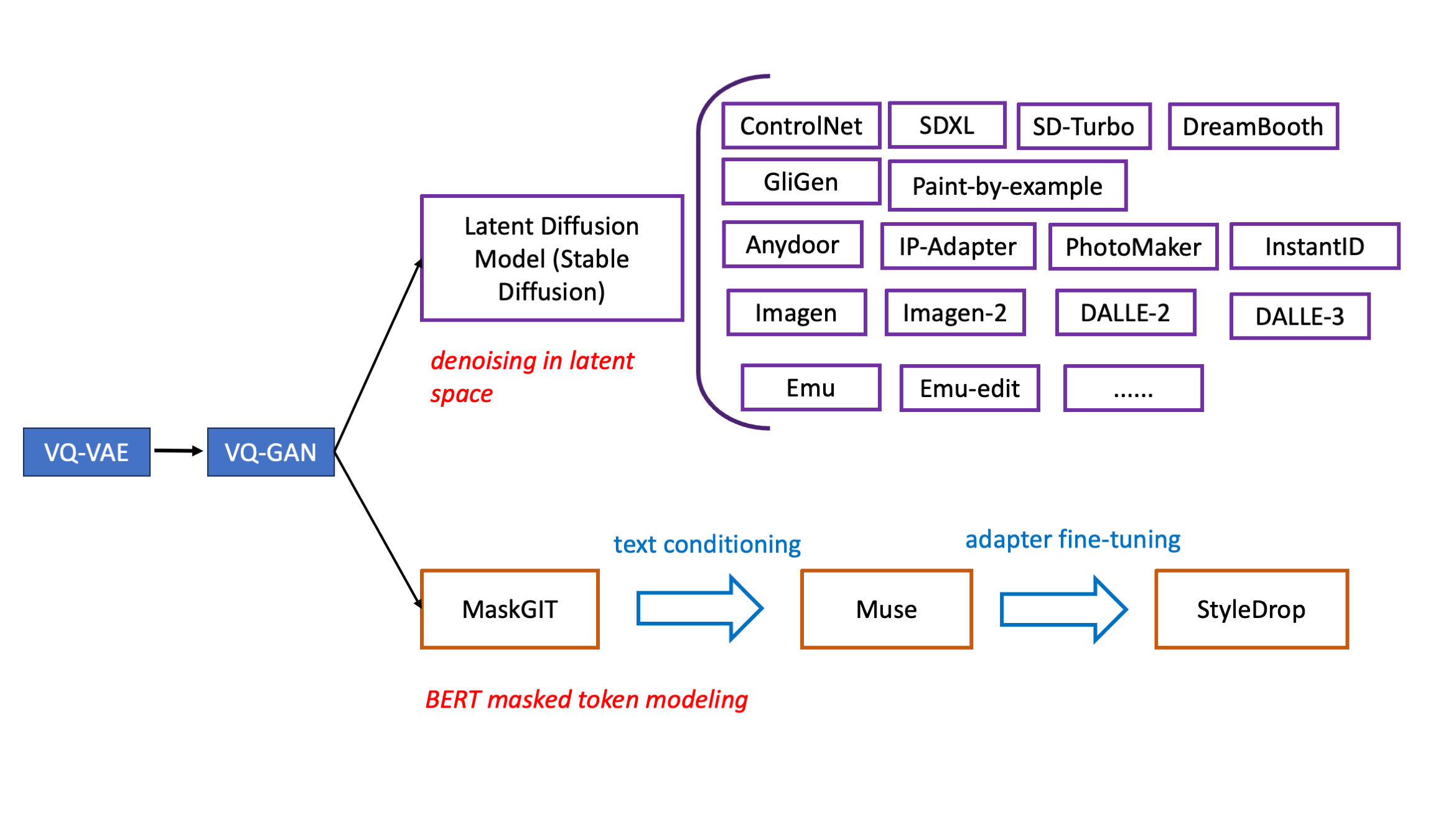
Two different approaches to image generation. Source: author
MaskGIT
MaskGIT ( Citation: Chang, Zhang & al., 2022 Chang, H., Zhang, H., Jiang, L., Liu, C. & Freeman, W. (2022). Maskgit: Masked generative image transformer. ) is an improvement over VQ-GAN. In VQ-GAN, tokens are modeled using a GPT-style autoregressive Transformer, which treats visual tokens as a 1D sequence and predicts the next token given previously generated tokens. In MaskGIT, this GPT model is substituted with a BERT model that predicts masked tokens. Note that MaskGIT is a foundational model trained mainly for unconditional image generation, which allows text-to-image models to be built upon it for incorporating more modalities and image editing applications.
Architecture
The model follows the same two-stage design as with VQ-GAN. First, an autoencoder is trained to learn to represent images with discrete tokens. Second, a BERT model is learnt to predict masked tokens. The purpose of the paper is to mainly investigate the second stage, so the first stage follows the same setup as in the VQ-GAN. MaskGIT Architecture. Source: paper
In theory, the model is able to infer all tokens and generate the entire image in a single pass. However, the authors found that this doesn’t work, so a gradual sampling procedure is employed, where at each step only predictions with high probabilities are retained, and others tokens are masked again.
A decreasing mask function $\gamma(r)\in(0,1]$ is used to mask tokens during training and inference. A number of functions are experimented, and linear and concave ones like cosine ($\cos x$), square ($1-x^2$), and cubic ($1-x^3$) are found to be the best ones. During training, a ratio $r$ is sampled from 0 to 1, then $\gamma(r)\cdot N$ tokens in $Y$ are uniformly selected for masking.
The decoding algorithm synthesizes an image in $T$ steps. At each iteration, the model predicts all tokens simultaneously but only keeps the most confident ones. The remaining tokens are masked out and re-predicted in the next iteration. The mask ratio is made decreasing until all tokens are generated within $T$ iterations. $T=8$ to $12$ iterations are found to yield best results.
Training
Loss. After the tokenizer is trained, a BERT model is trained to predict masked tokens. The training loss is cross entropy loss on masked tokens. $$ \mathcal{L} = -\mathbb{E}_{Y\in\mathcal{D}}\left[\sum_{\forall i\in[1, N], m_i=1}\log p\left(y_i\mid Y_{\overline{M}}\right)\right] $$ where $\mathcal{D}$ is dataset, $Y=[y_i]_1^N$ is image tokens with length $N$, $M=[m_i]_1^N$ is the corresponding binary mask.
Dataset. The model is trained on ImageNet 256x256 & 512x512 and Places2 dataset. For each dataset, a single autoencoder along with a codebook of 1024 tokens are trained.
Hardware. All models are trained on 4x4 TPU devices with a batch size of 256.
Code. List of implementations is available on paperswithcode.
Muse
Muse ( Citation: Chang, Zhang & al., 2023 Chang, H., Zhang, H., Barber, J., Maschinot, A., Lezama, J., Jiang, L., Yang, M., Murphy, K., Freeman, W., Rubinstein, M. & (2023). Muse: Text-to-image generation via masked generative transformers. arXiv preprint arXiv:2301.00704. ) is a text-conditioned MaskGIT model for real-world image generation application with numerous modifications over the original MaskGIT architecture. A 4.6B-parameter text encoder, T5-XXL, is used to map text prompts to 4096 dim embedding vectors that will be fused with token embeddings via cross attention. The image generation pipeline is split into two parts with a base module and a super-resolution module.
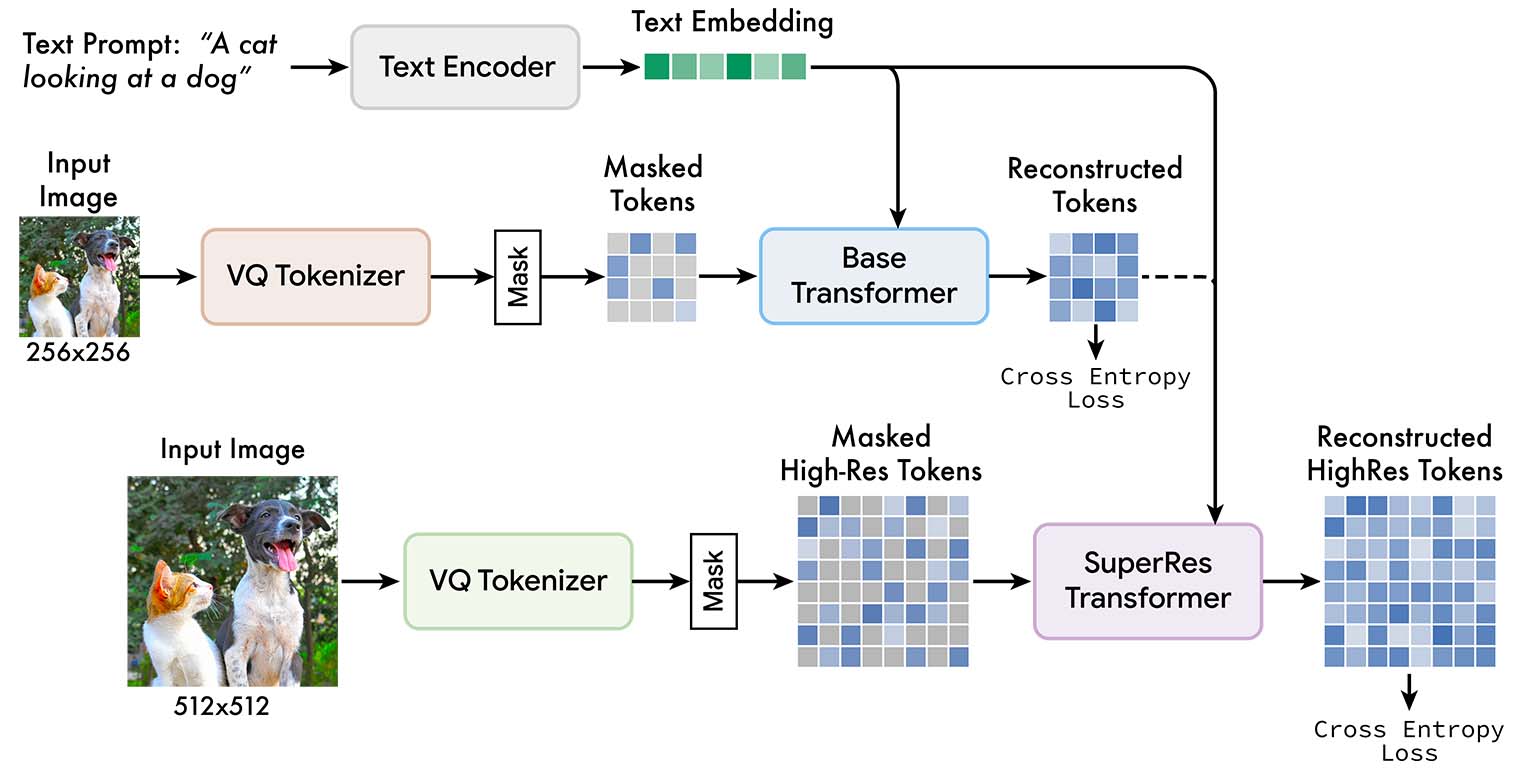
Muse Architecture. Source: paper
The reason for adding a super-resolution pipeline is that, directly predicting 512 × 512 resolution images is found to lead the model to focus on low-level details over large-scale semantics, yielding sup-optimal results. So a base model is first used to generate 16 × 16 latent embeddings (corresponding to 256 × 256 images), followed by a super-resolution model that upsamples base latent embeddings to 64 × 64 latent embeddings (corresponding to 512 × 512 images).
Low-resolution embeddings are passed into a series of self-attention transformer layers. The updated embeddings are concatenated with text embeddings. Then it is fused with high-resolution embeddings via cross-attention. In this way, the predicted high-resolution tokens take into account both its masked input as well as low-resolution tokens and text embeddings.
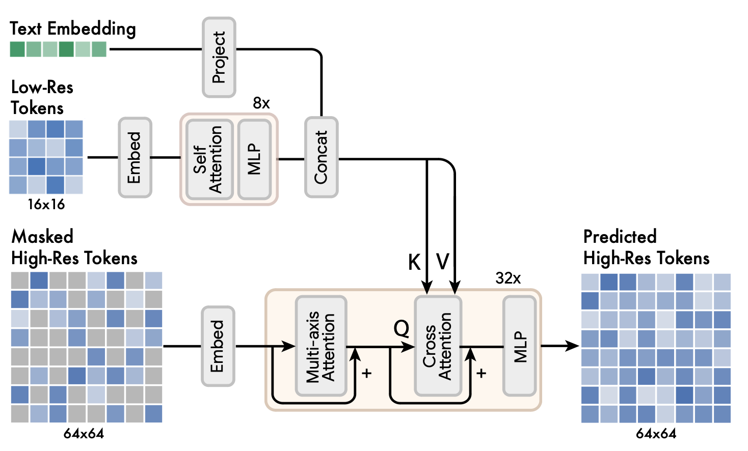
Muse super-resolution model. Source: paper
Besides super-resolution module, there are many other engineering designs over MaskGIT.
Decoder finetuning. To further improve the model’s ability to generate fine details, the VQ-GAN decoder is added with more layers and fine-tuned, while keeping the VQ-GAN encoder, codebook and transformers fixed.
Masking rate. As was done in MaskGIT, the model is trained with a variable masking rate, however the masking rate used in Muse is from a truncated $\arccos$ distribution with density function $p(r) = \frac{2}{\pi}(1-r^2)^{-1/2}$. The expectation of this distribution is $0.64$, with a bias towards higher masking rates. The authors claim that masking is not only critical for the sampling algorithm, but it also enables a number of zero-shot, out-of-the-box editing capabilities.
Classifier Free Guidance. At training time, text prompts in 10% of samples chosen randomly are removed, with image embedding self-attention substituted for text-image cross-attention. At inference time, a conditional logit $p_c$ and an unconditional logit $p_u$ are computed for each masked token. The final logits $p_g$ are formed by moving away from the unconditional logits by an amount $t$, the guidance scale: $$ p_g = (1 + t)\cdot p_c - tp_u. $$
This can also enable negative prompting: the user (or system) inputs negative prompts, then logit associated with the negative prompts $p_n$ replaces $p_u$ in above equation. This can be used to dissociate generated image tokens with negative prompts.
Training
- Dataset. 460 million text-image pairs from Imagen dataset.
- Model size. The tokenizer is a CNN model with 19 ResNet blocks with codebook of size 8192. A number of base transformer models at different sizes are trained, ranging from 600M to 3B parameters.
- Loss. The loss follows the same setup with MaskGIT. First, a VQ-GAN autoencoder is trained, with perception loss + GAN loss. Second, BERT is trained with NLL on masked tokens. The super-resolution model is trained after the base model has been trained.
- Hardware. The model is trained on 512-core TPU-v4 chips with a batch size of 512 for 1M steps, which takes about 1 week.
- Code.
Image Generation via Diffusions
Diffusion model was originally proposed in a paper titled “Deep unsupervised learning using nonequilibrium thermodynamics” ( Citation: Sohl-Dickstein, Weiss & al., 2015 Sohl-Dickstein, J., Weiss, E., Maheswaranathan, N. & Ganguli, S. (2015). Deep unsupervised learning using nonequilibrium thermodynamics. PMLR. ) , though the method per se does not depend on techniques in statistical mechanics.
To learn image generation, the method adds Gaussian noises to training data step by step, until they become almost complete noise at step $T$. The model is trained to predict denoised version of its input at any given step. For this reason, diffusion models are also called “denoising autoencoders”. Some methods make predictions of added noises only, instead of denoising their inputs.
Note that because there is an analytic formula for normal distribution, we don’t have to generate noisy training samples sequentially. We can directly compute noises needed to add to a training image at any step $t\in[0,\ldots,T]$ ( Citation: Ho, Jain & al., 2020 Ho, J., Jain, A. & Abbeel, P. (2020). Denoising diffusion probabilistic models. Advances in neural information processing systems, 33. 6840–6851. ; Citation: Song, Sohl-Dickstein & al., 2020 Song, Y., Sohl-Dickstein, J., Kingma, D., Kumar, A., Ermon, S. & Poole, B. (2020). Score-based generative modeling through stochastic differential equations. arXiv preprint arXiv:2011.13456. ) .

We don’t have to add small noises sequentially. Training data can be prepared in parallel and each sample can be computed in one step. Illustration from Song (2020).
Given the above explanation, the training objective is to minimize
$$ \ell = \mathbb{E}_{x, \epsilon\sim N(0,1), t}\| \epsilon_\theta(x_t, t) - \epsilon\|_2^2 $$
where $x$ are training samples, and $t$ is uniformly sampled from steps ${1, . . . , T }$.
Imagen
The Imangen model ( Citation: Saharia, Chan & al., 2022 Saharia, C., Chan, W., Saxena, S., Li, L., Whang, J., Denton, E., Ghasemipour, K., Gontijo Lopes, R., Karagol Ayan, B., Salimans, T. & (2022). Photorealistic text-to-image diffusion models with deep language understanding. Advances in Neural Information Processing Systems, 35. 36479–36494. ) is a pixel-space diffusion model. It is conceptually simple, with a frozen T5-XXL encoder to map text prompts to embeddings and a 64×64 image diffusion model, followed by two super-resolution diffusion models for generating 256×256 and 1024×1024 images. The U-Net backbone predicts denoised version of its input. All diffusion models are conditioned on text embeddings and use classifier-free guidance.
The 64×64 model has 2B parameters, the 256×256 model has 600M paramters, and the 1024×1024 model has 400M parameters. The models are trained with a batch size of 2048 on 256 TPU-v4 chips for 2.5M steps.
The authors reported that Imagen depends critically on classifier-free guidance for effective text conditioning.
In early days of diffusion models, to improve sample quality, a separate image classifier $p(c\mid z)$ is trained. Classifier-free guidance is an alternative technique that avoids this pretrained model by instead jointly training a single diffusion model on conditional and unconditional objectives via randomly dropping $c$ during training (e.g. with 10% probability). Sampling is performed using $$ \tilde{\epsilon}_\theta(z_t, c) = w\cdot\tilde{\epsilon}_\theta(z_t, c) + (1 − w)\cdot\tilde{\epsilon}_\theta(z_t). $$
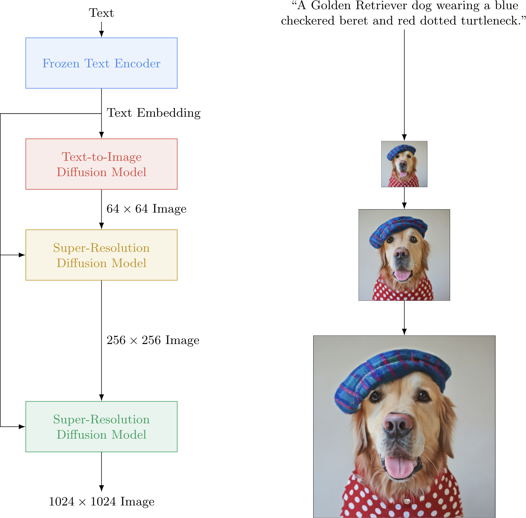
Imagen model architecture. Source: official website
Here are some open-source implementations of Imagen:
Latent Diffusion Model
Diffusion in pixel space is too expensive, because there are too many dimensions to keep track of: 512x512 color images have 512x512x3 = 786,432 dimensions, and 1024x1024 images have more than 3 million dimensions. In addition, information in pixel space is often very redundant, containing details that are not semantically important.
Latent Diffusion Models (LDM) ( Citation: Rombach, Blattmann & al., 2022 Rombach, R., Blattmann, A., Lorenz, D., Esser, P. & Ommer, B. (2022). High-resolution image synthesis with latent diffusion models. ) , also known as stable diffusion, map images to latent space with a trained autoencoder VQ-GAN $(\mathcal{E}, \mathcal{D})$, and learn U-Net backbones to reverse diffusions (noise-adding) in latent space. This has the benefit of reducing computational cost, and letting the model focus on semantics over details.
Note that the first author of LDM, Robin Rombach, is also the second author of VQ-GAN.
U-Net ( Citation: Ronneberger, Fischer & al., 2015 Ronneberger, O., Fischer, P. & Brox, T. (2015). U-net: Convolutional networks for biomedical image segmentation. Springer. ) is a convolutional neural network model that was first proposed to solve medical image segmentation task, where data size is small. For example, in the original paper, it was trained on a dataset of 30 images (512x512 pixels), and another dataset with 35 images. Recently, however, the U-Net backbone used in diffusion models is being replaced by the Transformer architecture.
An $H\times W\times 3$ image $x\in\mathbb{R}^{H\times W\times 3}$ will be mapped to $h\times w\times c$ latent tensor $z\in\mathbb{R}^{h\times w\times c}$. Some specific examples of $h\times w\times c$ are
- 64 x 64 x 3 (12,288 dims in total),
- 32 x 32 x 4 (4096 dims in total),
- 16 x 16 x 8 (2048 dims in total).
For conditional generation, text and image prompts are projected to vectors via an encoder $\tau_\theta$, then fused with U-Net intermediate layers via cross-attention. The loss is now
$$\ell = \mathbb{E}_{y, \epsilon\sim N(0,1), t}\| \epsilon_\theta(z_t, t, \tau_\theta(y)) - \epsilon\|_2^2.$$
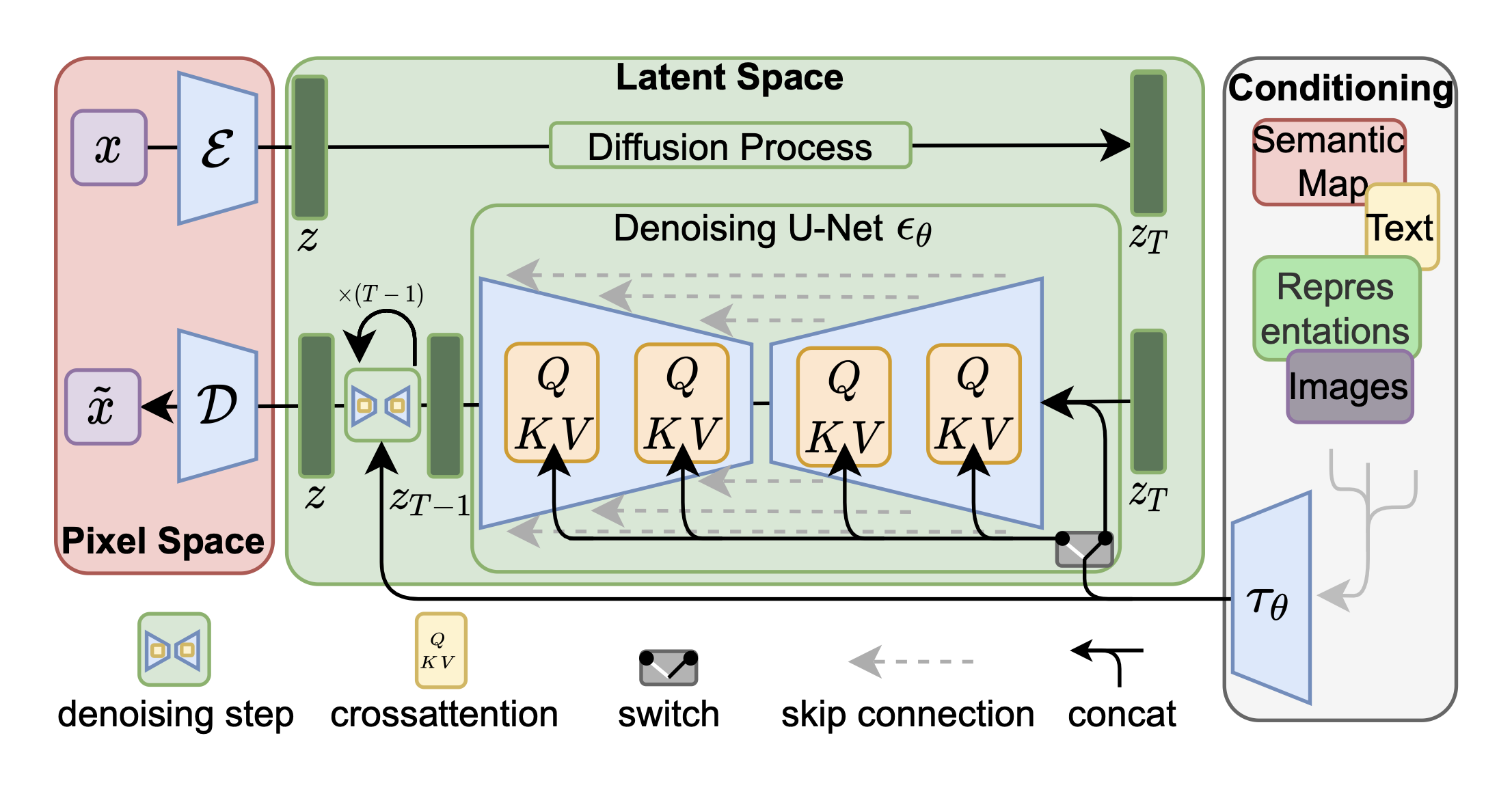
Latent Diffusion Model (LDM) architecture. Source: paper
ControlNet
ControlNet ( Citation: Zhang, Rao & al., 2023 Zhang, L., Rao, A. & Agrawala, M. (2023). Adding conditional control to text-to-image diffusion models. ) is an adapter-tuned stable diffusion model for generating images via image guidance like edge maps, human pose skeletons, segmentation maps, depth, and normals. For each of some U-Net blocks, specifically those encoder blocks, a trainable copy is added with zero convolution to process conditioning images and add the adapter output to the original block output.
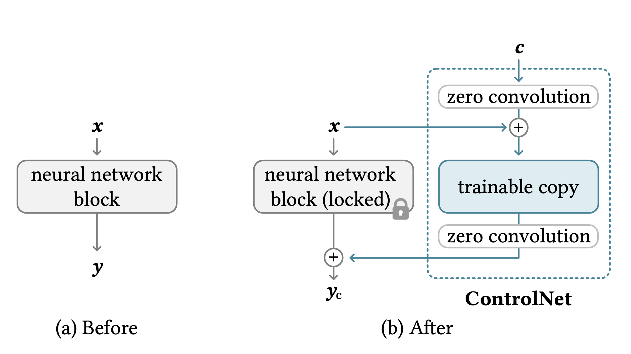
ControlNet architecture. Source: paper
The model is trained on (conditioning image, image) datasets, for example 3M canny edge image-caption pairs, 80K pose-image-caption pairs, 20K segmentation-image-caption pairs, 3M depth-image-caption pairs and more.
Weights & biases of the zero convolution (1x1 convolution) layers are initialized to zero, so at the start of training, the adapters output zero and the model outputs similar high quality images as the pre-trained SD model. The authors noted an interesting phenomenon of “sudden convergence”: the model suddenly learns to follow the input condition only at a certain training step.
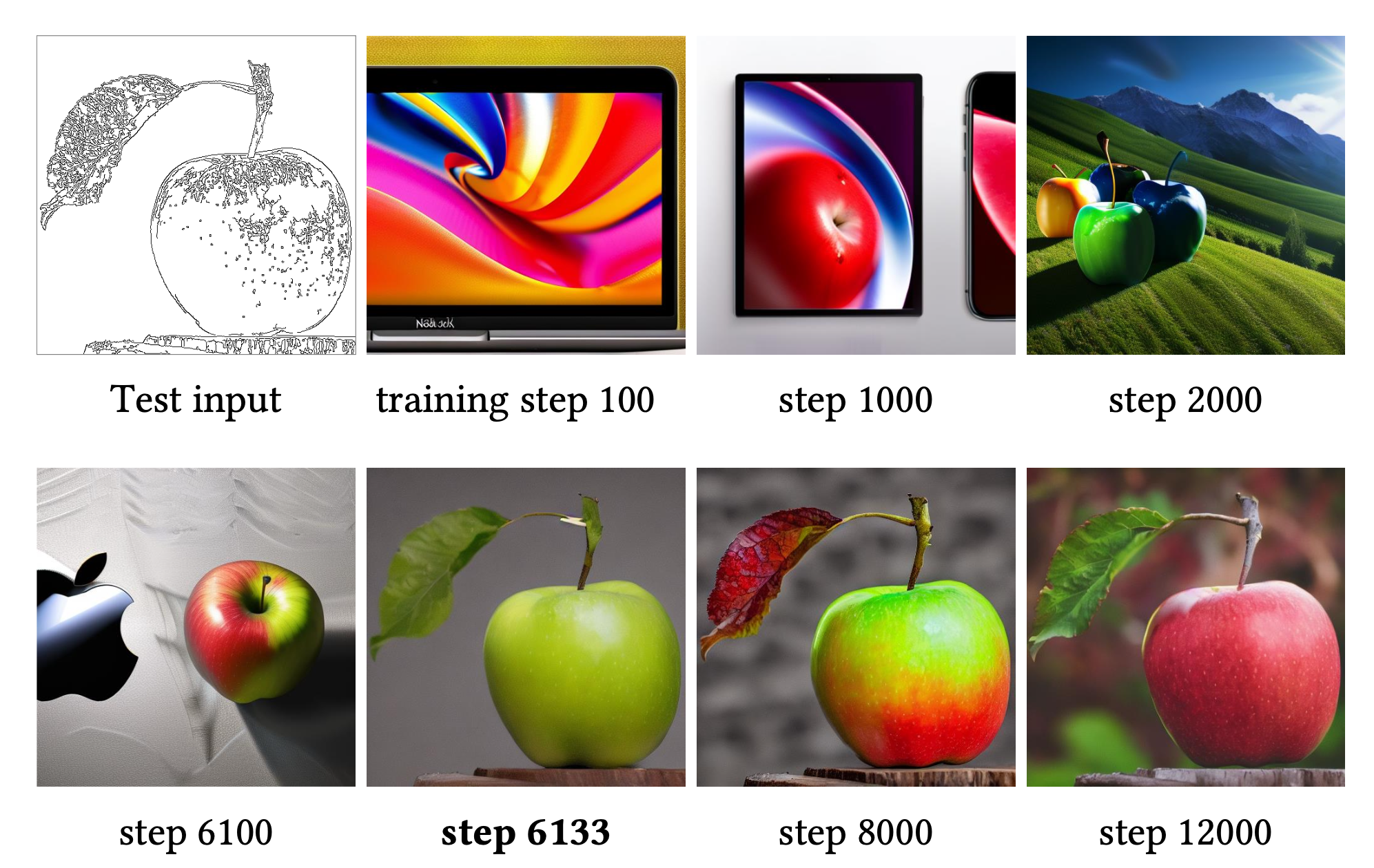
Sudden convergence phenomenon in ControlNet training. Source: paper
Anydoor
Anydoor ( Citation: Chen, Huang & al., 2023 Chen, X., Huang, L., Liu, Y., Shen, Y., Zhao, D. & Zhao, H. (2023). Anydoor: Zero-shot object-level image customization. arXiv preprint arXiv:2307.09481. ) is a fine-tuned stable diffusion model developed by researchers from Alibaba for placing objects in an image into another image at a specified location. It targets e-commerce applications:
- It can be used for placing a product into some desired background.
- Given an apparel as the object, and a model picture as the scene image, the model can place the cloth onto the model, generating try-on images.
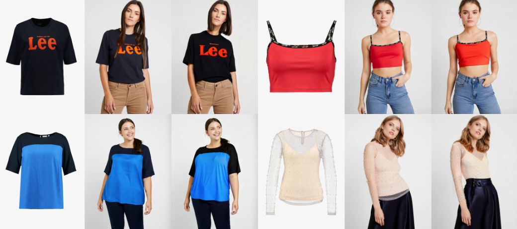
Anydoor can be applied to e-commerce tryon scenario
Architecture
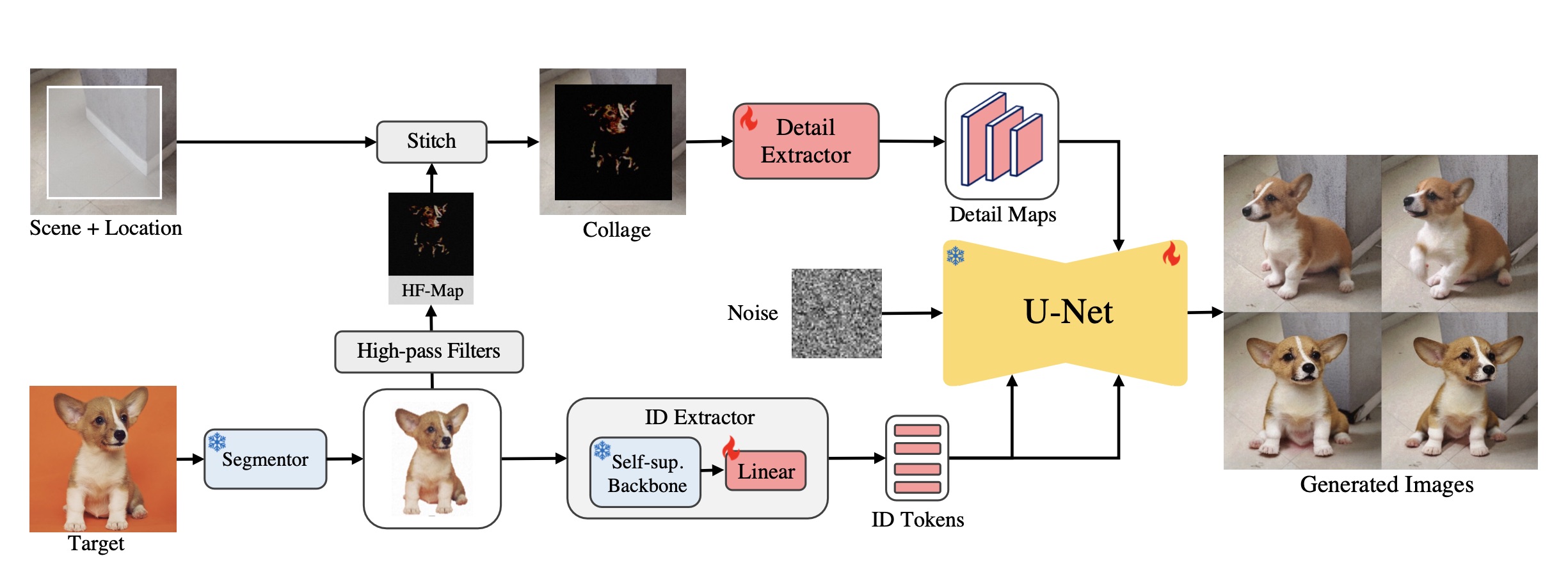
Anydoor model architecture. Source: paper
The architectural design is as follows: for the object image, first use a (freezed) segmentor model to remove the background, align the object to the image center, then feed the image to an ID extractor (freezed DINO-v2 + trainable linear layer) to extract the features as a $$ T^{257\times1024} = \mathrm{Linear}(T_g^{1\times1536}, T_p^{256\times1536}) $$ tensor, where $T_g^{1\times1536}$ is a global feature, and $T_p^{256\times1536}$ is a patch feature.
The extracted ID embeddings lack detail. To preserve high fidelity while also allow for diversity like gesture, lighting, and orientation, a high frequency map is used to extract fine details of the ID image: $$ I_h = (I\otimes K_h + I\otimes K_v) \odot I \odot M_{\mathrm{erode}} $$ where $K_h$ and $K_v$ are horizontal and vertical Sobel kernels, $\otimes$ is convolution, $\odot$ is Hadamard product (element-wise matrix multiplication), $M_{\mathrm{erode}}$ is an eroded mask used to filter out the information near the outer contour of the target object. See below for visualization of this transformation.
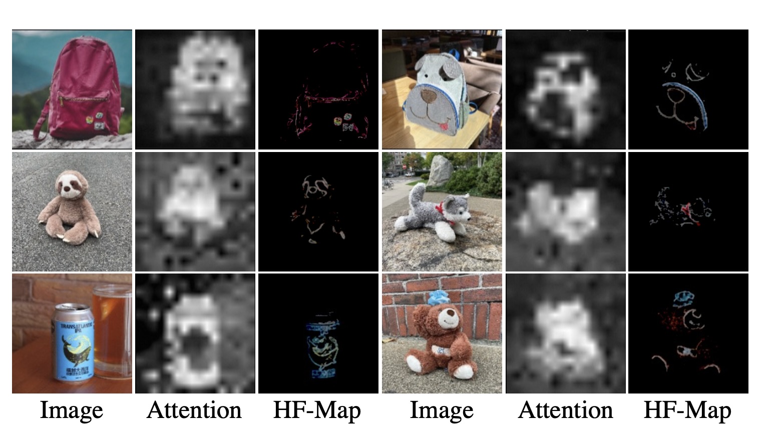
Visualization of HF maps
The HF-map is then stitched to the scene image at specified location, and a trainable detail extractor extracts features from the stitched image. The ID embeddings and the stitched image embeddings are then fused to the U-Net backbone via cross-attention. The model then output images that should be a harmonic composition of the object at the scene. The ID embeddings are injected into each U-Net layer, while the detail maps are concatenated with U-Net decoder features at each resolution. The U-Net encoder is freezed and only the U-Net decoder is trained.
Training
Dataset. The training data consists of 23,783 videos, 137,105 multi-view images, and 249,606 single-view images. The ideal training samples are image pairs for “the same object in different scenes”, which are difficult to obtain. To deal with this problem, the authors utilize video datasets to capture different frames containing the same object. Given a clip, the authors first sample two frames and segment the instances within each frame. Then, one instance from one frame is selected as the target object, and the same instance on the other frame is treated as the training supervision (i.e., the desired model output).
it is observed that initial denoising steps of a diffusion model often focus on generating the overall structure, while later steps cover fine details like textures and colors. Thus, video data is sampled with more chance in early denoising steps (large T) to better learn the appearance changes, and image data is sampled with more chance in late denoising steps (small T) to learn fine details.
Code. ali-vilab/AnyDoor
IP-Adapter
Given an input human face image and a prompt, the IP-Adapter model ( Citation: Ye, Zhang & al., 2023 Ye, H., Zhang, J., Liu, S., Han, X. & Yang, W. (2023). Ip-adapter: Text compatible image prompt adapter for text-to-image diffusion models. arXiv preprint arXiv:2308.06721. ) generates output image of that character under the scene described by the prompt. It is an adapter fine-tuned stable diffusion model. An Image encoder is added as trainable layers to process input images. Input image embeddings and text embeddings are fused via cross attention to the denoising U-Net backbone. The model has around 22M parameters.
Architecture
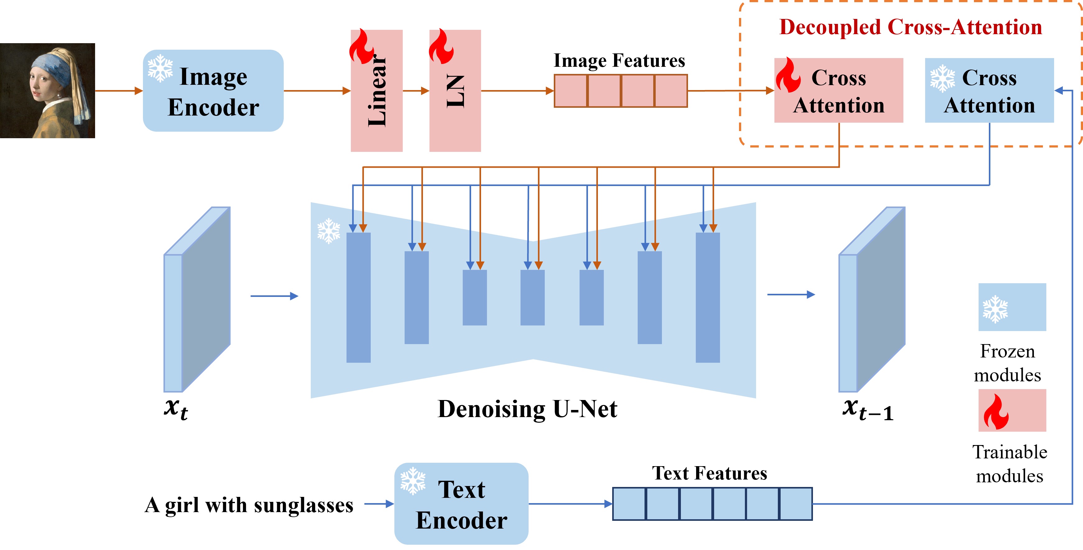
IP-Adapter model architecture. Source: paper
Training
- Loss. Same with stable diffusion, with classifier-free guidance.
- Dataset. 10M text-image pairs from two open source datasets, LAION-2B and COYO-700M. Images are resized to 512 × 512 resolution.
- Hardware. Trained on a single machine with 8 V100 GPUs for 1M steps.
- Code. tencent-ailab/IP-Adapter
PhotoMaker
As with IP-Adapter, the goal of the PhotoMaker model ( Citation: Li, Cao & al., 2023 Li, Z., Cao, M., Wang, X., Qi, Z., Cheng, M. & Shan, Y. (2023). PhotoMaker: Customizing realistic human photos via stacked ID embedding. arXiv preprint arXiv:2312.04461. ) is to re-draw the background and/or style described by text prompts while preserving the facial identity of a set of reference human images. Design of the model architecture comes from the observation that pre-trained CLIP models may associate words like “woman”, “man”, “girl” and “boy” to humans, and thus fusing those words’ embeddings with the image could guide the diffusion model to preserve the subject in the image.
After training, those models can output personalized image given an input reference image at reference time, without having to perform fine-tuning for each input instance. This is in contrast with earlier models like DreamBooth ( Citation: Ruiz, Li & al., 2023 Ruiz, N., Li, Y., Jampani, V., Pritch, Y., Rubinstein, M. & Aberman, K. (2023). Dreambooth: Fine tuning text-to-image diffusion models for subject-driven generation. ) , which fine-tunes diffusion model on each batch of reference images for personalization, which is expensive.
Architecture
A CLIP image encoder $\mathcal{E}_{img}$ is used to map $N$ human images supplied by the user to image embeddings $\{e^i\in\mathbb{R}^D\}_{i=1\ldots N}$, and a CLIP text encoder is used to map text prompt tokens of length $L$ to text embeddings $t\in\mathbb{R}^{L\times D}$. Non-human parts of input images are filled with noises to remove influence of the background, and additional trainable layers are added to the image encoder to fine-tune for such non-natural inputs.
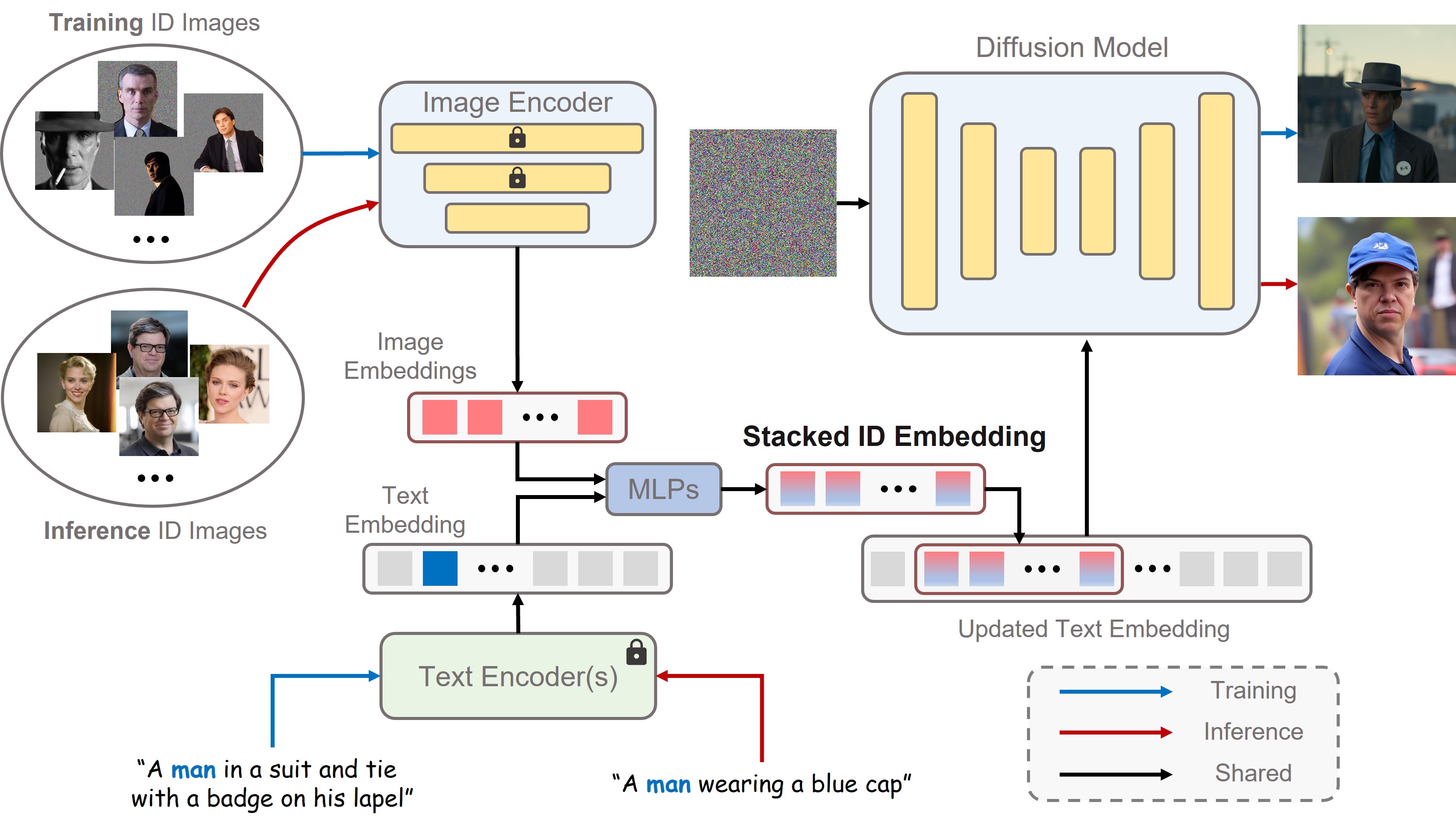
PhotoMaker model architecture
During inference, a “class” word from a set like {woman, man, girl, boy, young, old} is required in the text prompt. The text embedding $t_c\in\mathbb{R}^D$ that corresponds to the class word will be extracted and fused with each image embedding $e^i, i=1\ldots N$ through MLPs to get updated image embeddings $\{\hat{e}^i\in\mathbb{R}^D\}_{i=1\ldots N}$. We then concatenate them to get the concatenated embedding (called “stacked id embedding” in the paper) $$ s = (\hat{e}^1,\ldots,\hat{e}^N)\in\mathbb{R}^{N\times D}. $$
The conditional used to perform cross-attentions with the U-Net is defined as
$$ t^* = [t_1,\ldots, s, \ldots, t_L]\in\mathbb{R}^{(L-1 + N)\times D}. $$
Where $s$ replaces the vector corresponding to the class word $t_c$. Specifically, the cross-attention calculation is $$ Q = W_Q\cdot\phi(z_t) $$ $$ K = W_K\cdot t^* $$ $$ V = W_V \cdot t^* $$ $$ \text{Attention}(Q, K, V) = \text{softmax}\left(\frac{QK^T}{\sqrt{d}}\right)\cdot V $$ Attention matrices are fine-tuned by LoRA. The rest of the diffusion model remains unchanged.
Training
- Dataset. A dataset of 112K+ (image, caption, ID mask) triples of 13,000 people is collected, for an average of 8.6 pictures per person. The diffusion model used is SDXL ( Citation: Podell, English & al., 2023 Podell, D., English, Z., Lacey, K., Blattmann, A., Dockhorn, T., Müller, J., Penna, J. & Rombach, R. (2023). SDXL: Improving latent diffusion models for high-resolution image synthesis. arXiv preprint arXiv:2307.01952. ) , resolution of training data is 1024x1024.
- Hardware. The authors reported training on 8 Nvidia A100 GPUs for two weeks with a batch size of 48. For inference, a minimum of 15GB GPU memory is required.
- Test. The model shows impressive ability to preserve features presented in input image, like general facial shapes. But quite often the generated person is “different”. Rather, it looks like some kind of avarage of training images. In addition, there are noticeable artifacts in teeth and ears.

PhotoMaker test. The left one is the input image (Huiwen Chang). The middle one is generated with the prompt ‘an asian woman img sitting at the beach, with purple sunset’. The third one is generated with the prompt ‘An asian woman in front of a fountain at a garden img’. Source: author
- Code. TencentARC/PhotoMaker
